The AdventureWorks Database as a Transversal Matroid: Part I – Generating a Bipartite Graph
 September 18, 2011
Filed under Database, Mathematica
Tags: AdventureWorks, bipartite, Graph, Mathematica, Matroid, SQL

In previous posts, we took the foreign keys present in the AdventureWorks2008R2 database and used them to represent the database as a multigraph, a simple graph, and an incidence matrix. We even calculated properties such as graph radius and periphery. Another way to investigate relationships between objects is to present them as a matroid (or combinatorial pre-geometry).
To start, the simple graph of the finite key relationships present in the AdventureWorks database is already a cycle matroid. This is a very well known result as all finite graphs are cycle matroids. The independent sets in a cycle matroid are the edges that do not form a closed path. Arguably, the cycle matroid derived from the AdventureWorks database graph may have some interesting properties.
Instead of investigating the properties of this cycle matroid, we will investigate the AdventureWorks database as a transversal matroid. The definition of a transversal matroid in “Matroid Theory” by James Oxley is as follows:
A way to visualize transversals is via bipartite graphs:

The AdventureWorks database actually works as a great candidate for a transversal matroid. The family of subsets of the AdventureWorks database is the schemas. The AdventureWorks2008R2 database has the following schemas: dbo, HumanResources, Person, Production, Purchasing, and Sales. It’s easy to query the database for its schemas:
SELECT DISTINCT SCHEMA_NAME(schema_id) FROM sys.tables
The expected output is shown below.

To visualize the relationship between tables and schemas, we will need to create a bipartite graph of the relationship. We will create a connection to the database the usual way. Once that is accomplished, we will need to run the following command:

The reason we use CASE in the T-SQL statement is because there’s a table named Person too. So to take care of the fact that there’s a schema and a table of the same name, we just rename it. An partial listing of the output is show below:

We will need to combine the two columns into something Mathematica will like to work with for graphing.

I tried having the SQL query seamlessly put out columns of the form “SpecialOffer” -> “Sales”. While the query executed the way one would expect in SSMS, the parser Mathematica uses choked on it. So here we are, inelegantly combining the results. It is what it is. Perhaps I’ll find the trick.
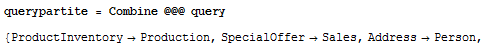
We apply the custom function Combine to the query result set.
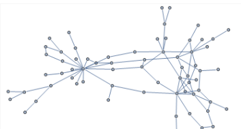
Finally, it’s time to see something worth looking at. The command below:

Returns:

To see the entire graph, click on the image. It’s very large.
While we’ve generated a great looking image of the relationship between schemas and tables in the AdventureWorks database, we have not yet described the matroid yet. In the second part of this series, we will generate the maximal independent sets to describe this matroid. I’m looking forward to it!
Graphing a Hierarchy from a Common Table Expression Using TreePlot
May 15, 2011
Filed under Mathematica, SQL Server
Tags: Common Table Expression, CTE, Microsoft SQL Server, Select (SQL), SQL, TreePlot
Common table expressions are one of the most underrated tools SQL Server ships with. CTEs greatly simplify querying SQL Server in situations where other queries would have either been extremely difficult or impossible to write. One can learn more about CTEs on MSDN. Further, I’d highly recommend this write-up by SQL Lion. It’s very thorough and provides a detailed breakdown of what is happening in a common table expression.
One of the great powers of CTEs is that they trivialize hierarchical queries. A common example is querying AdventureWorks to build a list of who reports to whom. Take the following query, shamelessly yanked from SQL Lion (with a tiny modification):
WITH EmpDetails (EmployeeKey, FirstName, LastName, ParentEmployeeKey,
PFirstName, PLastName, EmployeeRank, [Status])
AS
(
SELECT
EmployeeKey,FirstName,LastName,ParentEmployeeKey
,CAST('NULL' AS VARCHAR(50)) AS PFirstName
,CAST('NULL' AS VARCHAR(50)) AS PLastName
,1 AS EmployeeRank,[Status]
FROM dbo.DimEmployee
WHERE ParentEmployeeKey IS NULL
UNION ALL
SELECT e.EmployeeKey,e.FirstName,e.LastName,e.ParentEmployeeKey
,CAST(CTE_Emp.FirstName AS VARCHAR(50)) AS PFirstName
,CAST(CTE_Emp.LastName AS VARCHAR(50)) AS PLastName
,CTE_Emp.EmployeeRank + 1 AS EmployeeRank
,e.[Status]
FROM dbo.DimEmployee e
INNER JOIN EmpDetails CTE_Emp
ON e.ParentEmployeeKey = CTE_Emp.EmployeeKey
)
SELECT * FROM EmpDetails WHERE [Status] IS NOT NULL ORDER BY EmployeeRank
If we query the AdventureWorksDW2008R2 database, we should get a similar result to the result set below:
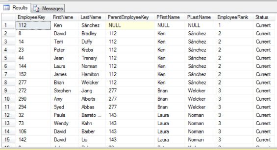
Reading the result set, we can see that Ken Sánchez reports to no one as his ParentEmployeeKey is NULL. Throughout the rest of the table, we can see we have individuals that have someone else they report to. In tabular format this is difficult to read and even harder to visualize.
Enter Mathematica and TreePlot[]. We want to take the essential data from the above output and create a visual representation. To start, we will want create a database connection in our notebook (.nb) file. This is done the usual way with DatabaseLink.

Take care to note that for the purposes of this example, we are connecting to the AdventureWorksDW2008R2 database and not AdventureWorks2008R2. Once connected, we will want to use the above query with a small modification.

We modified the SELECT * from the first query to SELECT EmployeeKey, ParentEmployeeKey. This is due to the fact that the other columns are extraneous to our purpose and will only create problems if we keep them in the result set. Once we run the command, we should receive a result set that appears as follows (the image is cropped):

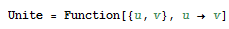
If we look at the TreePlot documentation, we note that our list isn’t quite in a usable state so we will have to massage the data some. The first thing we will do is define a function that will take two parameters u, v, and return u -> v. To do this, we will use the Function[] function in the following manner: Unite = Function[{u,v}, u -> v]
I’ve named my function Unite. It’s a terrible name. Feel free to name yours better. Once the function is built, we need to apply it to the list. To do this, we will use Apply[].

We’ve used shorthand here with the three @ signs. The reason we’ve done so is that the default behavior of Apply would be to apply the “Unite” function at the top level of the list. We want it to apply at one level beneath that. The three @@@ signs is shorthand for doing exactly that. The documentation for Apply discusses it. Also note that the Apply function stripped the sublists out of the list, giving us a litany of relation rules ready for TreePlot. To use TreePlot, merely pass the variable for the relation rules and any options needed. In this example, we want to label our vertices.

It appears that we have four discrete trees in our hierarchy! While this would seem to be unexpected, a simple verification of the data does show that this is not inaccurate. The trees are quite small and very busy so if we select them, click, and drag, we can see them in better detail.


That’s it! We’ve just used a common table expression to query a database for hierarchical relationships and then used Mathematica to graph it. Play around with it and leave any comments you might have. Thanks for reading.
Using SSIS to Loop Over Result Set and Dynamically Generate Output Files
April 9, 2011
Filed under BIDS, SSIS
Tags: BIDS, Control Flow, Foreach Loop Container, ResultSet, Select (SQL), SQL, SQL Server Integration Services, SSIS
This post is inspired largely by Ken Simmons’ excellent primer at SQLServerCentral.com. All I’ve done is extend it to a full result set.
Scenario: Let’s suppose one of the more successful sales partners at your organization created a slick spreadsheet in Excel that tracks key performance indicators. After a meeting, the entire department wants their own individual CSV so they can build a spreadsheet that looks exactly like hers. With some quick work in SSIS, it’s possible to deliver a unique CSV for each person.
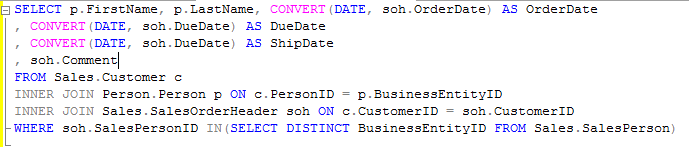
The sales department wants to tracks orders along with customers, perhaps something like the query below:
We will want only the customers for whom the sales person has an order with to get included in the sales person’s spreadsheet. To start, we will begin as Ken Simmon’s article begins. In your SSIS project, drag an Execute SQL Task from the toolbox into the control flow.

Right click and edit the task. Set the ResultSet to, “Full Result Set”. In the SQL Statement section, make sure your ConnectionType is set to OLE DB and click on new connection.

Build out your connection as you normally would to the AdventureWorks database. Mine looks like the following:

Click the ellipses next to SQLStatement and put in the following query, “SELECT DISTINCT CONVERT(NVARCHAR(4), Sales.BusinessEntityID) AS BusinessEntityID FROM Sales.SalesPerson”:

Next, click the Result Set section in the Execute SQL Task Editor and click the, “Add” button, select, “New Variable, and create a variable as the one below. Set the Result Name to the number zero (0) and give it a variable name. Mine is User::SalesPersonResultSet.

Add another variable. I named mine SalesPersonID and gave it a type of string. Package scope here is important. The scope is set to package so that both the Foreach Loop and the Data Task will be able to use the same variable.

Drag out a Foreach Loop Container onto the Control Flow:

Edit the Foreach Loop Container and click on the, “Collection” section. Set your enumerator to, “Foreach ADO Enumerator”, select the ADO object source variable to be User::SalesPersonResultSet, and the default value of, “Rows in the first table” suffices for this example.

Next, click on Variable Mappings and add the User::SalesPersonID. Here we’re taking each value that is encountered in User:SalesPersonResultSet and setting it to User:SalesPersonID. The Data Task will then operate on SalesPersonID until the Foreach Loop ends.

Drag a Dataflow Task out and drop it into the Foreach Loop Container. Once you’ve done that, click on the Data Flow tab.

Click and drag an OLD DB Source out onto the Data Flow Task and edit it. Your connection manager screen should look like the following:

Click the Parameters button and modify it so it looks like the below:

Click, “Okay” until you’re back to the Data Flow Task tab. Drag out a Flat File Destination, and we’ll build it out much like Ken Simmons did in his article. Create a new Flat File Connection and set it up something like the following:

Next, click on the properties for the Flat File Connections and click on the, “Expressions” ellipses. Set your Property to ConnectionString and build your expression as it shows below:

Once that is done, it’s time to try it out. Click, “OK” until you’re back at the package and click the, “Play” button.

We check the output destination:

And we check the files themselves:

That’s it. I know the post is a little long. There’s lots that can be expanded upon. For example, we can try to change the package to output directly to Excel spreadsheets. I have not done this myself so I don’t know how much of the package must be changed to do so. That might make for a good follow up post. Another thing to do is change the output of the first query to have the sales person’s full name instead of BusinessUnitID, since no one would really find that user friendly. Thanks for reading!
